Moving load
Load that changes in time

Pantograph

Train

Rifle
Examples of a moving load.
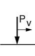
Force
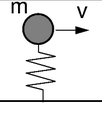
Oscillator
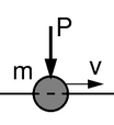
Mass
Types of a moving load.
In structural dynamics, a moving load changes the point at which the load is applied over time.[citation needed] Examples include a vehicle that travels across a bridge[citation needed] and a train moving along a track.[citation needed]
Properties
In computational models, load is usually applied as
- a simple massless force,[citation needed]
- an oscillator,[citation needed] or
- an inertial force (mass and a massless force).[citation needed]
Numerous historical reviews of the moving load problem exist.[1][2] Several publications deal with similar problems.[3]
The fundamental monograph is devoted to massless loads.[4] Inertial load in numerical models is described in [5]
Unexpected property of differential equations that govern the motion of the mass particle travelling on the string, Timoshenko beam, and Mindlin plate is described in.[6] It is the discontinuity of the mass trajectory near the end of the span (well visible in string at the speed v=0.5c).[citation needed] The moving load significantly increases displacements.[citation needed] The critical velocity, at which the growth of displacements is the maximum, must be taken into account in engineering projects.[citation needed]
Structures that carry moving loads can have finite dimensions or can be infinite and supported periodically or placed on the elastic foundation.[citation needed]
Consider simply supported string of the length l, cross-sectional area A, mass density ρ, tensile force N, subjected to a constant force P moving with constant velocity v. The motion equation of the string under the moving force has a form[citation needed]

Displacements of any point of the simply supported string is given by the sinus series[citation needed]

where

and the natural circular frequency of the string

In the case of inertial moving load, the analytical solutions are unknown.[citation needed] The equation of motion is increased by the term related to the inertia of the moving load. A concentrated mass m accompanied by a point force P:[citation needed]


The last term, because of complexity of computations, is often neglected by engineers.[citation needed] The load influence is reduced to the massless load term.[citation needed] Sometimes the oscillator is placed in the contact point.[citation needed] Such approaches are acceptable only in low range of the travelling load velocity.[citation needed] In higher ranges both the amplitude and the frequency of vibrations differ significantly in the case of both types of a load.[citation needed]
The differential equation can be solved in a semi-analytical way only for simple problems.[citation needed] The series determining the solution converges well and 2-3 terms are sufficient in practice.[citation needed] More complex problems can be solved by the finite element method[citation needed] or space-time finite element method.[citation needed]
| massless load | inertial load |
|---|---|
  |   |
The discontinuity of the mass trajectory is also well visible in the Timoshenko beam.[citation needed] High shear stiffness emphasizes the phenomenon.[citation needed]

The Renaudot approach vs. the Yakushev approach
Renaudot approach
- [citation needed]
![{\displaystyle \delta (x-vt){\frac {\mbox{d}}{{\mbox{d}}t}}\left[m{\frac {{\mbox{d}}w(vt,t)}{{\mbox{d}}t}}\right]=\delta (x-vt)m{\frac {{\mbox{d}}^{2}w(vt,t)}{{\mbox{d}}t^{2}}}\ .}](https://wikimedia.org/api/rest_v1/media/math/render/svg/16ed1fb87ff883ac7a361c5654fe90e8d55a9333)
Yakushev approach
- [citation needed]
![{\displaystyle {\frac {\mbox{d}}{{\mbox{d}}t}}\left[\delta (x-vt)m{\frac {{\mbox{d}}w(vt,t)}{{\mbox{d}}t}}\right]=-\delta ^{\prime }(x-vt)mv{\frac {{\mbox{d}}w(vt,t)}{{\mbox{d}}t}}+\delta (x-vt)m{\frac {{\mbox{d}}^{2}w(vt,t)}{{\mbox{d}}t^{2}}}\ .}](https://wikimedia.org/api/rest_v1/media/math/render/svg/5dd5e7ef47ac9717cecc4d848a1b89250fee1baf)
Massless string under moving inertial load
Consider a massless string, which is a particular case of moving inertial load problem. The first to solve the problem was Smith.[7] The analysis will follow the solution of Fryba.[4] Assuming ρ=0, the equation of motion of a string under a moving mass can be put into the following form[citation needed]

We impose simply-supported boundary conditions and zero initial conditions.[citation needed] To solve this equation we use the convolution property.[citation needed] We assume dimensionless displacements of the string y and dimensionless time τ:[citation needed]


where wst is the static deflection in the middle of the string. The solution is given by a sum

where α is the dimensionless parameters :

Parameters a, b and c are given below


In the case of α=1, the considered problem has a closed solution:[citation needed]
![{\displaystyle y(\tau )=\left[{\frac {4}{3}}\tau (1-\tau )-{\frac {4}{3}}\tau \left(1+2\tau \ln(1-\tau )+2\ln(1-\tau )\right)\right]\ .}](https://wikimedia.org/api/rest_v1/media/math/render/svg/b4b742b059c127a4e38555987978d29ed35b7668)
References
- ^ Inglis, C.E. (1934). A Mathematical Treatise on Vibrations in Railway Bridges. Cambridge University Press.
- ^ Schallenkamp, A. (1937). "Schwingungen von Tragern bei bewegten Lasten". Ingenieur-Archiv (in German). 8 (3). Stringer Nature: 182–98. doi:10.1007/BF02085995. S2CID 122387048.
- ^ A.V. Pesterev; L.A. Bergman; C.A. Tan; T.C. Tsao; B. Yang (2003). "On Asymptotics of the Solution of the Moving Oscillator Problem" (PDF). J. Sound Vib. Vol. 260. pp. 519–36. Archived from the original (PDF) on 2012-10-18. Retrieved 2012-11-09.
- ^ a b Fryba, L. (1999). Vibrations of Solids and Structures Under Moving Loads. Thomas Telford House. ISBN 9780727727411.
- ^ Bajer, C.I.; Dyniewicz, B. (2012). Numerical Analysis of Vibrations of Structures Under Moving Inertial Load. Lecture Notes in Applied and Computational Mechanics. Vol. 65. Springer. doi:10.1007/978-3-642-29548-5. ISBN 978-3-642-29547-8.
- ^ B. Dyniewicz & C.I. Bajer (2009). "Paradox of the Particle's Trajectory Moving on a String". Arch. Appl. Mech. 79 (3): 213–23. Bibcode:2009AAM....79..213D. doi:10.1007/s00419-008-0222-9. S2CID 56291972.
- ^ C.E. Smith (1964). "Motion of a stretched string carrying a moving mass particle". J. Appl. Mech. Vol. 31, no. 1. pp. 29–37.


